In 2018, Uber AI Labs developed a new layer for the deep learning practitioner: CoordConv. This concept was explained and tested in their paper and a simpler summary was also provided in the form of a blog post. 

Both of these are very accessible and I highly recommend them for those wishing to see how this layer improves performance on a range of problems. For the purposes of this tutorial however, I'll be going over the specifics of the code for implementing this layer and applying it to 3 of the problems mentioned in the original work. Before I dive into that, I'll give a brief explanation of what CoordConv is so that you can follow along with the code without having to read the entirety of the aforementioned blog post or paper.

The Failing of Convolutions on 3 Simple Problems

Convolutions are ubiquitous in modern deep learning architectures. One of their supposed strengths is their translational invariance; regardless of where a feature is present in an image, the same feature template can be applied. Using the same feature template across the image also helps reduce the number of parameters which results in easier training. However, translational invariance may not always be helpful. As the developers of CoordConv show, the normal convolutional approach is unable to solve 3 seemingly simple tasks that revolve around translation between the Cartesian space and the one-hot coordinate space:

• Supervised Rendering: Given some Cartesian coordinate (i,j), highlight a 9x9 patch on a64x64 canvas centered around the provided coordinate.
• Supervised Coordinate Classification: Given some Cartesian coordinate (i,j), provide its corresponding one-hot vector representation for a vector of size 4096.
• Supervised Regression: Given a one-hot vector of length 4096, provide its corresponding Cartesian coordinate representation in the 64x64 space.

Normal convolutions perform very poorly; we'll examine some results later on.

CoordConv Layer

The proposed solution is to:

...allows filters to know where they are in Cartesian space by adding extra, hard-coded input channels that contain coordinates of the data seen by the convolutional filter.

For a 2D image with I rows and J columns, two extra feature channels are added with the following entries: for the first channels, the 0th row just contains 0s, the next row just contains all 1s, while for the second channels, the 0th column just contains 0s, the next contains all 1s (i.e. the coordinates of the pixels are being supplied). This is what the additional channels look like at the input layer. For other layers in the network, the number of rows and columns will correspond to the height and width of the feature map at that particular layer instead. So CoordConv can be applied at any layer, not just the input layer (which is really the only one working in the raw pixel space). Figure 1 below provides a visual representation of CoordConv. Another channel that can be introduced is the distance of that particular pixel from the centre of the image, a polar coordinate representation.

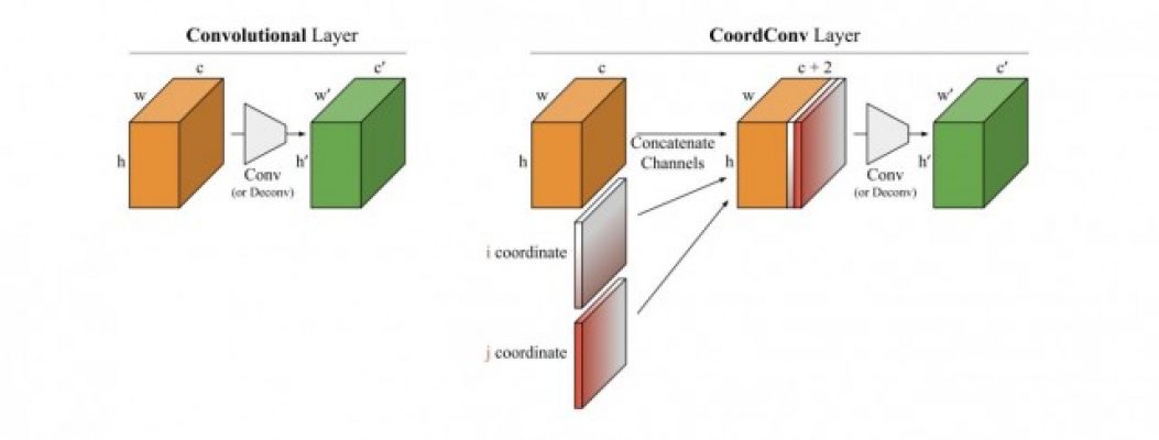Figure 1 (sourced from Figure 3 of the original CoordConv paper): A visual explanation of how the coordconv layer differs from a normal convolution layer.

Maintaining the Benefits of Convolution

Two of the main benefits gained from using convolutions are the reduction in parameters and the translation parameter. Adding extra channels will increase the number of parameters. However, as the authors note in the paper:

a standard convolutional layer with square kernel size k and with c input channels and c' output channels will contain cc'k^2 weights, whereas the corresponding CoordConv layer will contain (c + d)c'k^2 weights, where d is the number of coordinate dimensions used (e.g. 2 or 3).

d is 2 when we only consider the Cartesian channels and 3 when we introduce the polar coordinate channel. From the above, we can see that the increase in number of parameters is manageable. Furthermore, for those who are interested, the authors describe a way of reducing the increase in the number of parameters by using a separate filter for the coordinate channels (see footnote 2 in the original paper). For the purposes of the experiments we'll be working through, we'll use the first method which is slightly easier to implement.

Regarding the translational invariance, it's important to note that because we are introducing the coordinate data via concatenated channels, the convolutional filters can learn to ignore these if these channels are not helpful for the task the network is trying to solve. In fact, if the network learns to assign weights of 0s to the parameters interacting with these channels, then the behaviour of the filters is as if we were simply using normal convolutions and not CoordConv. Hence, we can view the normal convolution input as a subset of CoordConv, one that can be learned if appropriate for the task. Although for the experiments we will look at, we will be able to see how beneficial it can be to have these extra channels if the task at hand requires them.

Code

Let's dive into how you can implement CoordConv. I've taken the following from the original paper but I think it's worth going through the various lines to better understand how the whole block ends up functioning as what I've described above. Additionally, I've made a couple of edits to the overall wrapper compared to what you might encounter in the paper. They chose to implement it as a function of a class but I found that to be a tad overkill so I stripped it down to a simple function.

All the code I discuss in this paper can be found here, my implementation of coordconv. Additionally, this repository also contains code for running experiments to compare the the coorconv vs non-coordconv methods on the classification, regression, and rendering tasks. Please feel free to dive into it and play around with it yourself. If you notice any issues, do open up a pull request and I'll see to it as soon as I can!

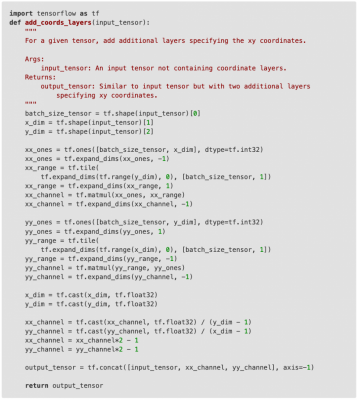
That might look slightly intimidating but I'll go through the different sections and explain what's going on. To help us ground this code, let's assume that our input tensor has a shape of [8, 28, 30, 3]. So this could be a collection of 8 images of height 28, width 30, with 3 colour channels (e.g. red, green, blue).

Getting Tensor Information

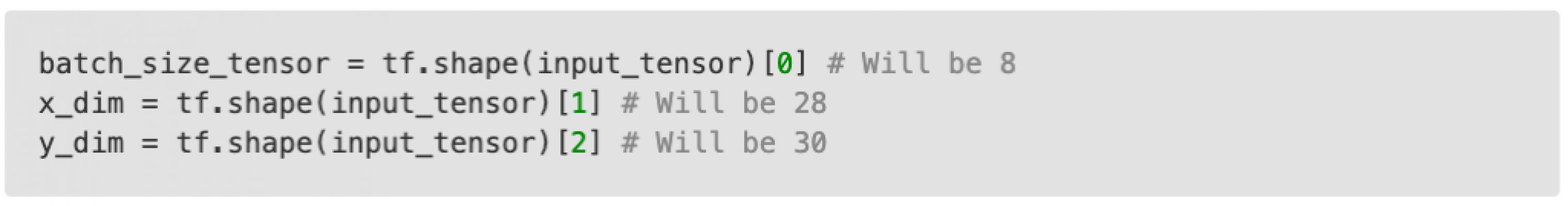
These initial lines fetch the different dimensions of the tensor: the batch size, the number of rows, and the number of columns.

An Array of Ones

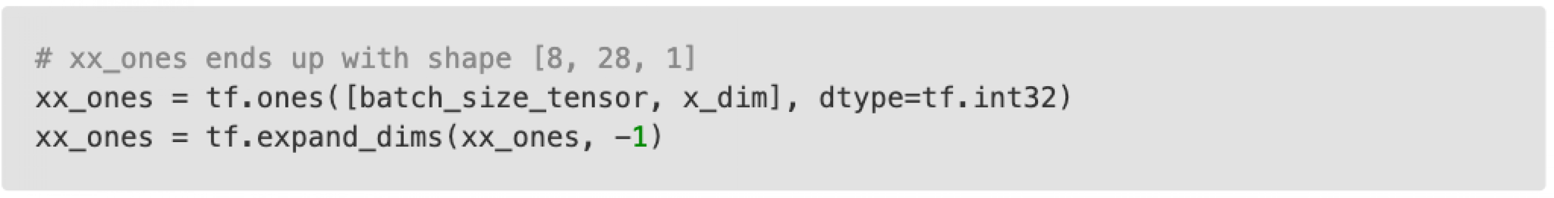
We first create an array of ones with shape [8, 28] and then add on an extra dimension at the end.

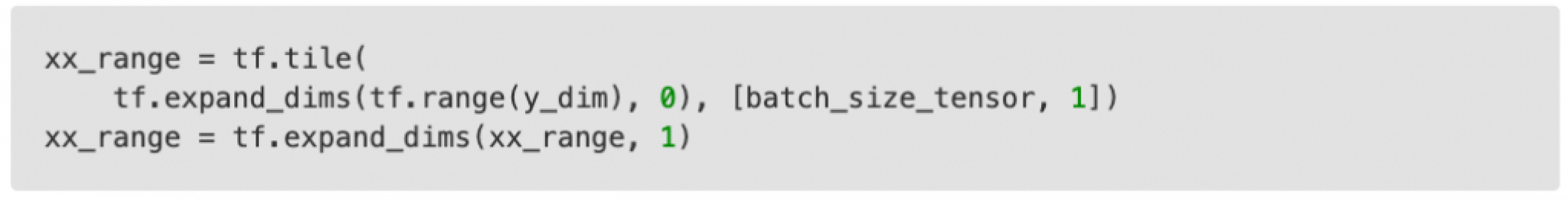
I think this is probably the most complicated bit, especially the tile call so let's go through it in more detail. First we have the tf.range(y_dim) call and this creates a vector like so: [0 1 ... 29]. It just has the same number of rows as y_dim, the width of the image and a single entry in each row, an index denoting which row we are presently at. The tf.expand_dims call then changes this vector to [[0 1 ... 29]]: an additional dimension is introduced at the front so now the shape of the array is (1, 29). Next, we have the tf.tile call which took me the longest to understand. We've already been through what the first argument to this call is. The second argument dictates how many times the first argument should be repeated (or tiled) along each axis. So along the first axis, we want the first argument (the array [[0 1 ... 29]]) repeated batch_size_tensor (here 8) times. Along the second axis, don't repeat the array. To understand how it could be repeated along the second, if instead of 1, we specified 2, then along each element of the batch, the tensor would hold [[0 1 ... 29 0 1 .. 29]]. The tf.expand_dims call here inserts a dimension at axis 1 so the final shape of the tensor is (8, 1, 30).

Putting it together

Here we combine our previous tensors of shape (8, 28, 1) and (8, 1 30) to have the almost final channel of (8, 28, 30). We will want to concatenate this later on with our original tensor which had 4 dimensions so once again we use tf.expand_dims to add a final dimension.

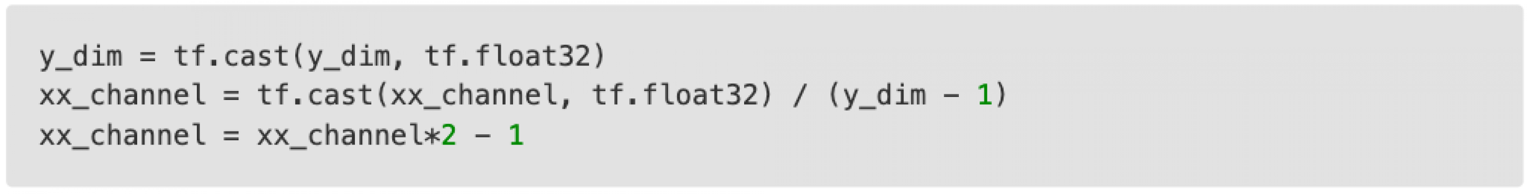
Scaling

The second maps the coordinates we have onto the range [0, 1] and the third line further maps that to [-1, 1]. Casting to floats is required because up to this point we've been working with integers but now we require decimals. If you plan to work with images a lot, this snippet is a handy one to remember as we often want the network inputs to be in the range [-1, 1]. To finish it all off, we concatenate our new x-channel, y-channel, and original input tensor.

I won't go through the computation for the y-channel but hopefully, it's clear how that functions.

P.S.

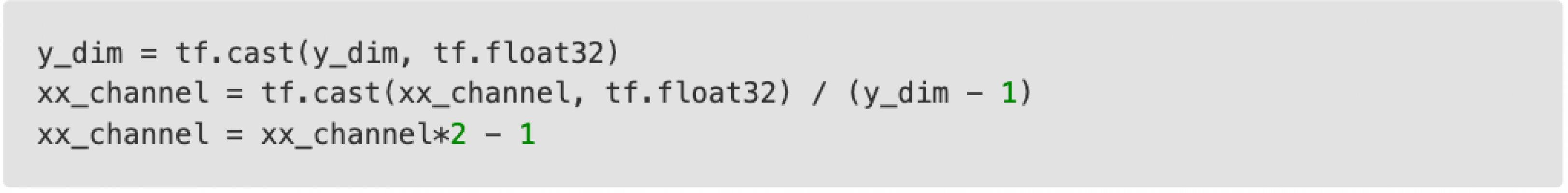
For those of you who look at the original paper and the code snippet they provided, you might notice that the line involving the mapping to [0, 1] has a minute difference compared to mine. Instead of dividing by (y_dim - 1), they divide by (x_dim - 1). Since the channel consists of coordinates from 0 to y_dim, we need to be dividing by the y dimension, not x, so their computation is incorrect! The only scenario where this would be equivalent is when we are working with square inputs and y_dim = x_dim. Coincidentally, that represents the input in a majority of their experiments which is perhaps why this small bug wasn't picked up.

Dataset

We'll be looking at the supervised rendering and supervised coordinate classification task. Both these tasks are essentially the reversed of each other and utilize the same Not-so-Clevr dataset. This dataset consists of 9x9 squares on a 64x64 canvases. Each square is linked to a cartesian coordinate, the center point of the square. Building on what I mentioned in the introduction, the rendering tasks involves translating from the Cartesian coordinate space to the 64x64 canvas and the classification task translates from a 64x64 canvas with a single 9x9 patch highlighted back to the Cartesian coordinate space.

To highlight the simplicity of their dataset, the original authors note that the bulk of the dataset can be generated in two lines of code:

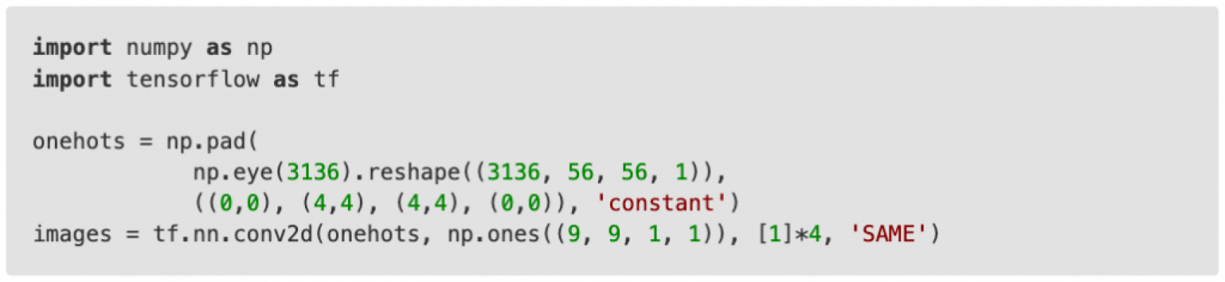
While it does only involve 2 lines, they are quite packed so I'll provide a brief explanation here. The np.eye command creates a identity matrix of size 3136x3136. If we consider each row of the identity matrix, only one entry is 1 while all the others are 0. Thus we can consider this matrix a collection of all the one-hot vectors for the vector length 3136. The np.reshape command takes each of our one-hot vectors and converts it to a 56x56x1 array. If we think about this array as a 56x56 canvas and consider that each was reshaped from a different one-hot vector, then we can see that for each of the 3136 56x56 canvases, there will only be a single pixel highlighted while all the others are 0. Next they use np.pad to enlarge the size of each canvas. The first and last (0,0) parameters indicate that there shouldn't be any padding on the first dimension (the one of size 3136) or the last (the one of size 1). The middle two (4,4) pad the other two dimensions by 4 zeros on each side so the resulting array now has shape (3136, 64, 64, 1). Going back to the idea of canvases, now each of the 3136 entries is a canvas of size 64x64 with a single entry highlighted on the smaller grid of 56x56. The tensorflow 2d convolution that follows applies a 9x9 filter of 1s to each pixel of each canvas. Whenever it encounters a 0 on the canvas, nothing changes but when it encounters the single highlighted 1 per canvas, a 9x9 grid of 1s is now formed, centered around the original 1. Thus we arrive at 9x9 patches on a canvas of 64x64.

Alongside these, the experiments also require a set of Cartesian coordinates but the code to do so is much simpler so I won't go through it here.

The remaining piece with regards to the dataset is how the examples were split between the training and testing subsets. The authors propose the following two options:

• Uniform: 80% of the examples are randomly selected to be in the training set and the remaining 20% are assigned to the test set.
• Quadrant: The data is broken up into 4 quadrants. 3 of the quadrants are assigned to the training set and the remaining quadrant is the test set.

The choice of split is quite important because for some of the experiments, the normal convolution is able to achieve passable results when applied to the uniform split but does extremely poorly for the quadrant split. The CoordConv layer however does well on both.

Architecture for each task

My implementations for each of these architectures can be found here. I provide the instructions for running the experiments on the repository and the settings you require are noted here, for each experiment. Please feel free to try it yourself and experiment around. This will definitely push your learning along more than simply reading this tutorial.

Supervised Coordinate Classification

The architecture details for the models used for classification are provided in the first section of the supplementary material of the original paper. For the experiment using normal convolutions, the input to the network is the pair of Cartesian coordinates and a series of transposed convolutions is then applied to this to upscale to a 64x64 map with a single-pixel highlighted. When using the CoordConv layer, the Cartesian Coordinate input is tiled to produce a 64x64 grid, the CoordConv layer is added to this feature map, and then a series of convolutions is applied to produce the 64x64 grid with a single-pixel highlighted. For all cases, a cross-entropy loss is used.

One aspect of this setup that initially confused me was why one approach used transposed convolutions and the other used regular convolutions. Before sitting down to properly think this through, I tried tiling the Cartesian coordinates to create the 64x64 grid, NOT adding the CoordConv layer, and then applying normal convolutions to see what would happen. What happens in this scenario is that every part of the input that the convolutional filters look at are exactly the same and hence the struggles extremely hard to learn. However, when using the transposed convolutions to scale up the Cartesian coordinates to a 64x64 grid, each item on the grid is slightly different and this facilitates better learning. This issue doesn't have to be dealt with when using the CoordConv layer because in that scenario, the added feature maps ensure differences across the grid.

Supervised Regression

The architecture details for the models used for regression are provided in the third section of the supplementary material of the original paper. It is interesting to note that when using CoordConv, the network is significantly simpler and applicable to both the uniform and test split. However, two different architectures had to be developed when relying on normal convolutions and the authors note that while the network for the uniform split was quite robust to changes in the hyperparameters, the network for the quadrant split was delicate with regards to hyperparameters. This once again highlights the inability of normal convolutions to learn the correct generalization for this task. For all the architectures here, a mean squared error loss was used.

For the CoordConv architecture, I did find that there were a couple of 'required' settings for the hyperparameter to ensure that the network properly learned the task. Firstly, when the authors say to use global pooling at the last layer, it is important to use max-pooling and not average-pooling. Use of the latter leads to network to constantly predict the coordinate [31.5, 31.5]. That it is a float is not the issue; this can be simply remedied by rounding up or down. However, this was the prediction regardless of the input and a quick glance shows that the network is simply predicting the 'average' coordinate of each axis. I think this is because the act of average-pooling is essentially a forced act of translation invariance and so the specificity provided by CoordConv is lost. The other hyperparameter that I found necessary was a sufficiently large learning rate. If I used a value of say 1e-4, the network once again had the same prediction issue. In this instance, I postulate that these predictions are part of a local minimum that is difficult to exit with lower learning rates. Learning rates of 1e-3 or even 1e-2 enabled the network to produce correct predictions. Another aspect that could lead to this pitfall was training for too long. For both the uniform and quadrant split, I found that almost perfect predictions were made within 5-10 epochs. Training for longer caused the network to once again start predicting the average coordinate pair. I would guess that that particular good, local minimum is not very large and further training with the high learning rate forces the network to the other bad, local minimum that is more difficult to leave.

Supervised Rendering

For this task, the architectures used when dealing with normal convolutions and CoordConv versions are very similar to their supervised coordinate classification. The main difference is that the more channels are used at each stage. Furthermore, instead of using a standard cross-entropy loss, where only a single-pixel is targeted for highlighting, the rendering tasks utilized a per-pixel cross-entropy loss, thus enabling highlighting of a 9x9 grid.

Results

While the original paper and the blog post both provided plenty of results, I'll show you the results I got using the code I wrote which you can access and run yourself. This way, you can more easily verify the different claims for yourself. If you'd like, you're also free to play with the architectures and hyperparameters yourself to see if you can obtain interesting or better results.

For each task, we'll compare the results of using normal convolutions vs including the CoordConv maps on both the uniform and quadrant splits. All tasks used a batch size of 32.

Supervised Coordinate Classification

CoordConv

Deconv

Supervised Regression

CoordConv

Conv

Discussion: Classification and Regression

CoordConv achieved perfect performance on all the tasks here with minimal effort whereas the methods that did not utilize coordconv fared poorly in a lot of the cases, even after I spent a significant amount of time trying to tune the hyperparameters to achieve better results. The large gap between the uniform and quadrant splits for the non coordconv methods indicate that there is probably over-fitting going on hence why when assessed on data outside the training distribution, the methods perform very poorly.

Supervised Rendering

For these experiments, instead of considering accuracy, a visual inspection is more helpful.

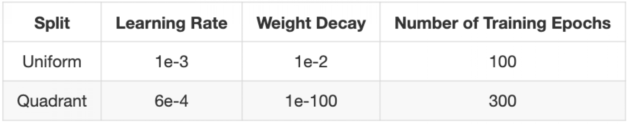
For both data splits, I used the same hyperparameters for both the coordconv and the deconv method. Here are the settings:

CoordConv

Uniform data split, training examples:

Uniform data split, testing examples:

Quadrant data split, training examples:

Quadrant data split, testing examples:

Deconv

Uniform data split, training examples:

Uniform data split, testing examples:

Quadrant data split, training examples:

Quadrant data split, testing examples:

Discussion: Rendering

The results here were not what I expected. Based on the performance on the other tasks and the results presented in the original paper, I thought I would be able to achieve near-perfect performance on this when using coordconv but as you can see from above this was not the case, especially on the quadrant test split.

One thing I did notice though was that when I terminated training for the coordconv methods, the loss was still decreasing, albeit very slowly. Hence I hypothesize that given more training steps or a better learning schedule, the coordconv method may be able to render much cleaner boxes.

If we look at the results from the deconv methods however, there is some evidence that more training would not help. For the uniform data split, we see that the boxes have very messy boundaries, even during training. Poor training performance is not reassuring when really we are interested in achieving good test performance. If we consider the quadrant split, the performance on the training subset is near perfect, even better than the coordconv method. However, this is in stark contrast to the performance of the test subset. This indicates that the model used its capacity to over-fit onto the training subset. More training would likely only exacerbate this issue.

Discussion

Coordconv definitely helped achieve better results for the different experiments I tried above. Even for the uniform data split, I found that when using coordconv, it took much less time to find good hyperparameters. Furthermore, for the experiments above, I only used coordconv at the input layer though you can apply it at any layer of the networks or even to several layers.

There have been some criticisms of the CoordConv layer. One that I found quite insightful and even fun to read was Piekniewski's Autopsy Of A Deep Learning Paper. While I agree with some of their points, based on my experience both in these experiments and in an industrial setting, I would still recommend trying out the coordconv layers. It is relatively cheap to implement and even if it doesn't help improve the final objective you're optimizing for, it might make it easier to choose hyperparameters.

Keep in mind that coordconv most benefits tasks that could do with more localized information and less translation invariance. However, the way coordconv is being used means that the network can decide how much importance the coordconv features should be assigned.

Conclusion

I hope that you have gained a useful addition to your deep learning tool kit. If you haven't already, do go play with the repository as that will definitely help you solidify your understanding and knowledge.

References

[1] Liu, R., Lehman, J., Molino, P., Such, F.P., Frank, E., Sergeev, A. and Yosinski, J., 2018. An Intriguing Failing of Convolutional Neural Networks and the CoordConv Solution. arXiv preprint arXiv:1807.03247.

[2] Uber Blog Post: An Intriguing Failing of Convolutional Neural Networks and the CoordConv Solution

[3] Autopsy Of A Deep Learning Paper

Further tutorials to practice your skills on:

- Introduction to Missing Data Imputation
- Six Data Science projects to expand your skills and knowledge
- Unit testing with PySpark
- Hyperparameter tuning in XGBoost
- Getting started with XGBoost

Ashwin D. D’Cruz is a Machine Learning Engineer at Calipsa. He holds an MPhil in Machine Learning, Speech and Language Technology.