Nowadays, recommender systems are used to personalize your experience on the web, telling you what to buy, where to eat or even who you should be friends with. People's tastes vary, but generally follow patterns. 

People tend to like things that are similar to other things they like, and they tend to have similar taste as other people they are close with. Recommender systems try to capture these patterns to help predict what else you might like. E-commerce, social media, video and online news platforms have been actively deploying their own recommender systems to help their customers to choose products more efficiently, which serves win-win strategy.

Two most ubiquitous types of recommender systems are Content-Based and Collaborative Filtering (CF). Collaborative filtering produces recommendations based on the knowledge of users’ attitude to items, that is it uses the "wisdom of the crowd" to recommend items. In contrast, content-based recommender systems focus on the attributes of the items and give you recommendations based on the similarity between them.

In general, Collaborative filtering (CF) is the workhorse of recommender engines. The algorithm has a very interesting property of being able to do feature learning on its own, which means that it can start to learn for itself what features to use. CF can be divided into Memory-Based Collaborative Filtering and Model-Based Collaborative filtering. In this tutorial, you will implement Model-Based CF by using singular value decomposition (SVD) and Memory-Based CF by computing cosine similarity.

We will use MovieLens dataset, which is one of the most common datasets used when implementing and testing recommender engines. It contains 100k movie ratings from 943 users and a selection of 1682 movies. You should add unzipped movielens dataset folder to your notebook directory. You can download the dataset here.

You read in the u.data file, which contains the full dataset. You can read a brief description of the dataset here.

Get a sneak peek of the first two rows in the dataset. Next, let's count the number of unique users and movies.

You can use the scikit-learn library to split the dataset into testing and training. Cross_validation.train_test_split shuffles and splits the data into two datasets according to the percentage of test examples (test_size), which in this case is 0.25.

Memory-Based Collaborative Filtering

Memory-Based Collaborative Filtering approaches can be divided into two main sections: user-item filtering and item-item filtering. A user-item filtering will take a particular user, find users that are similar to that user based on similarity of ratings, and recommend items that those similar users liked. In contrast, item-item filtering will take an item, find users who liked that item, and find other items that those users or similar users also liked. It takes items and outputs other items as recommendations.

• Item-Item Collaborative Filtering: “Users who liked this item also liked …”
• User-Item Collaborative Filtering: “Users who are similar to you also liked …”

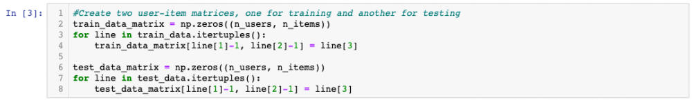
In both cases, you create a user-item matrix which you build from the entire dataset. Since you have split the data into testing and training you will need to create two [943 x 1682] matrices. The training matrix contains 75% of the ratings and the testing matrix contains 25% of the ratings.

After you have built the user-item matrix you calculate the similarity and create a similarity matrix.

The similarity values between items in Item-Item Collaborative Filtering are measured by observing all the users who have rated both items.

For User-Item Collaborative Filtering the similarity values between users are measured by observing all the items that are rated by both users.

A distance metric commonly used in recommender systems is cosine similarity, where the ratings are seen as vectors in n-dimensional space and the similarity is calculated based on the angle between these vectors. Cosine similiarity for users a and m can be calculated using the formula below, where you take dot product of the user vector 
u k

 and the user vector 
u a

 and divide it by multiplication of the Euclidean lengths of the vectors.

To calculate similarity between items m and b you use the formula:

Your first step will be to create the user-item matrix. Since you have both testing and training data you need to create two matrices.

You can use the pairwise_distances function from sklearn to calculate the cosine similarity. Note, the output will range from 0 to 1 since the ratings are all positive.

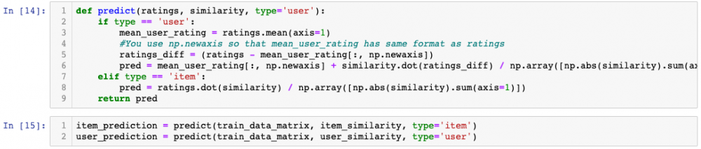
Next step is to make predictions. You have already created similarity matrices: user_similarity and item_similarity and therefore you can make a prediction by applying following formula for user-based CF:

You can look at the similarity between users k and a as weights that are multiplied by the ratings of a similar user a (corrected for the average rating of that user). You will need to normalize it so that the ratings stay between 1 and 5 and, as a final step, sum the average ratings for the user that you are trying to predict.

The idea here is that certain users may tend always to give high or low ratings to all movies. The relative difference in the ratings that these users give is more important than the absolute rating values. To give an example: suppose, user k gives 4 stars to his favourite movies and 3 stars to all other good movies. Suppose now that another user t rates movies that he/she likes with 5 stars, and the movies he/she fell asleep over with 3 stars. These two users could have a very similar taste but treat the rating system differently.

When making a prediction for item-based CF you don't need to correct for users average rating since query user itself is used to do predictions.

Describing Data

Evaluation

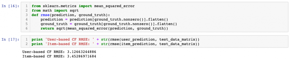
There are many evaluation metrics but one of the most popular metric used to evaluate accuracy of predicted ratings is Root Mean Squared Error (RMSE).

You can use the mean_square_error (MSE) function from sklearn, where the RMSE is just the square root of MSE. To read more about different evaluation metrics you can take a look at this article.

Since you only want to consider predicted ratings that are in the test dataset, you filter out all other elements in the prediction matrix with prediction[ground_truth.nonzero()].

Memory-based algorithms are easy to implement and produce reasonable prediction quality. The drawback of memory-based CF is that it doesn't scale to real-world scenarios and doesn't address the well-known cold-start problem, that is when new user or new item enters the system. Model-based CF methods are scalable and can deal with higher sparsity level than memory-based models, but also suffer when new users or items that don't have any ratings enter the system.

Model-based Collaborative Filtering

Model-based Collaborative Filtering is based on matrix factorization (MF) which has received greater exposure, mainly as an unsupervised learning method for latent variable decomposition and dimensionality reduction. Matrix factorization is widely used for recommender systems where it can deal better with scalability and sparsity than Memory-based CF. The goal of MF is to learn the latent preferences of users and the latent attributes of items from known ratings (learn features that describe the characteristics of ratings) to then predict the unknown ratings through the dot product of the latent features of users and items. When you have a very sparse matrix, with a lot of dimensions, by doing matrix factorization you can restructure the user-item matrix into low-rank structure, and you can represent the matrix by the multiplication of two low-rank matrices, where the rows contain the latent vector. You fit this matrix to approximate your original matrix, as closely as possible, by multiplying the low-rank matrices together, which fills in the entries missing in the original matrix.

Let's calculate the sparsity level of MovieLens dataset:

To give an example of the learned latent preferences of the users and items: let's say for the MovieLens dataset you have the following information: (user id, age, location, gender, movie id, director, actor, language, year, rating). By applying matrix factorization the model learns that important user features are age group (under 10, 10-18, 18-30, 30-90)_, _location and gender_, and for movie features it learns that _decade_, _director and actor are most important. Now if you look into the information you have stored, there is no such feature as the _decade_, but the model can learn on its own. The important aspect is that the CF model only uses data (user_id, movie_id, rating) to learn the latent features. If there is little data available model-based CF model will predict poorly, since it will be more difficult to learn the latent features.

Models that use both ratings and content features are called Hybrid Recommender Systems where both Collaborative Filtering and Content-based Models are combined. Hybrid recommender systems usually show higher accuracy than Collaborative Filtering or Content-based Models on their own: they are capable to address the cold-start problem better since if you don't have any ratings for a user or an item you could use the metadata from the user or item to make a prediction. Hybrid recommender systems will be covered in the next tutorials.

SVD

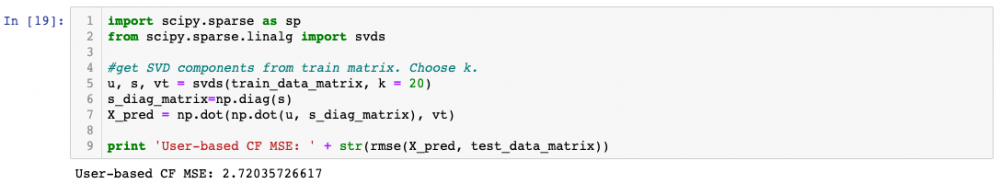
A well-known matrix factorization method is Singular value decomposition (SVD). Collaborative Filtering can be formulated by approximating a matrix X by using singular value decomposition. The winning team at the Netflix Prize competition used SVD matrix factorization models to produce product recommendations, for more information I recommend to read articles: Netflix Recommendations: Beyond the 5 stars and Netflix Prize and SVD. The general equation can be expressed as follows:

Given m x n matrix X:

• U is an (m x r) orthogonal matrix
• S is an (r x r) diagonal matrix with non-negative real numbers on the diagonal
• V^T is an (r x n) orthogonal matrix

Elements on the diagnoal in S are known as singular values of X.

Matrix X can be factorized to U, S and V. The U matrix represents the feature vectors corresponding to the users in the hidden feature space and the V matrix represents the feature vectors corresponding to the items in the hidden feature space.

Now you can make a prediction by taking dot product of U, S and V^T.

Carelessly addressing only the relatively few known entries is highly prone to overfitting. SVD can be very slow and computationally expensive. More recent work minimizes the squared error by applying alternating least square or stochastic gradient descent and uses regularization terms to prevent overfitting. You can see one of our previous [tutorials] on stochastic gradient descent for more details. Alternating least square and stochastic gradient descent methods for CF will be covered in the next tutorials.

To wrap it up:

• In this post we have covered how to implement simple Collaborative Filtering methods, both memory-based CF and model-based CF.
• Memory-based models are based on similarity between items or users, where we use cosine-similarity.
• Model-based CF is based on matrix factorization where we use SVD to factorize the matrix.
• Building recommender systems that perform well in cold-start scenarios (where litle data is availabe on new users and items) remains a challenge. The standard collaborative filtering method performs poorly is such settings. In the next tutorials you will have the change to dig deeper into this problem.

ABOUT THE AUTHOR: Agnes Johannsdottir

Agnes is a master student in Business Analytics at University College London. She studied Management Engineering in Iceland and worked for 2 years as an IT consultant in supply chain. Her main interests lie in using data science methods (especially machine learning) to apply in Retail and Supply Chain businesses.

Subscribe to Our Newsletter

Subscribe now to receive our bi-weekly Data Science newsletter featuring industry news, interviews, tutorials, popular resources to develop your skills and much more!