


Regression analysis is one of the approaches in the Machine Learning toolbox. It is widely used in many fields but its application to real-world problems requires intuition for posing the right questions and a substantial amount of “black art” that can't be found in textbooks. While practice and experience are required to develop these intuitions, there are practical steps that you can take to get started.
This article provides you with a starting point by showing you how to build a regression model from raw data and assess the quality of its predictions. The article will use code examples in Python. Before running the code make sure you have the following libraries installed: pandas, matplotlib and sklearn.
Imagine you are working for a bike sharing company that operates in the area of a specific city. This company has a bike sharing scheme where users are able to rent a bike from a particular location and return it at a different location using the machines at the parking spots. You are in charge of predicting how many bikes are going to be used in the future. This is obviously very important for predicting the revenues of the company and planning infrastructure improvements. Unfortunately, you don’t know much about bike sharing. All you have been given is a csv file where you have the number of bikes hired every day.
You can import the file with Python using pandas and check the first five lines:
import pandas as pd

bikes = pd.read_csv('bikes.csv')

bikes.head()| date | temperature | humidity | windspead | count | |
|---|---|---|---|---|---|
| 0 | 2011-01-03 | 2.716070 | 45.715346 | 21.414957 | 120 |
| 1 | 2011-01-04 | 2.896673 | 54.267219 | 15.136882 | 108 |
| 2 | 2011-01-05 | 4.235654 | 45.697702 | 17.034578 | 82 |
| 3 | 2011-01-06 | 3.112643 | 50.237349 | 10.091568 | 88 |
| 4 | 2011-01-07 | 2.723918 | 49.144928 | 15.738204 | 148 |
Here you notice that not only you have the number of bikes hired for each day, but also the average weather condition in that day. At this point it's worth checking if there's a relation between the weather and the bikes used. Plot the temperature against the bike count to find out:
from matplotlib import pyplot as plt
plt.figure(figsize=(8,6))
 plt.plot(bikes['temperature'], bikes['count'], 'o')
 plt.xlabel('temperature')
 plt.ylabel('bikes')
 plt.show()
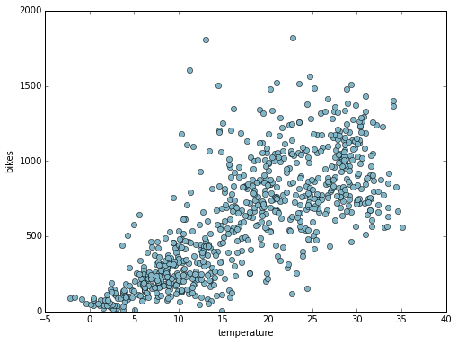
Scatter plot
Bingo! Here you see that there is a clear relation between the number of bikes hired and temperature. You have observed that as the temperature increases, the number of bikes hired generally increases too. However, how can you use this information to predict the number of bikes hired? This is where regression analysis comes in our help. With regression analysis you can capture the relationship between temperature and number bikes hired in a model that you can query any time you need to estimate the number of bikes from the temperature.
There are many regression techniques that you can apply; the one that you will use here is called Decision Trees. Why?
- It is a rule based technique. The prediction is done by applying a cascade of rules of the type “is the temperature less or equal than x degrees?”. This makes the model easy to interpret.
- It doesn’t require any data transformation. It means that we don’t have to spend more time preprocessing the data.
- It can handle complex relationships (not only simple linear relationships).
sklearn provides an implementation of the Decision Trees which is very straightforward to use:
from sklearn.tree import DecisionTreeRegressor

import numpy as np
regressor = DecisionTreeRegressor(max_depth=2)
 regressor.fit(np.array([bikes['temperature']]).T, bikes['count'])
Here we instantiated the regressor and, calling the method fit, we optimised (in technical terms trained) it for our data. Now you can answer questions such as “how many bikes will be hired when the temperature is 5 degrees?”
<code class="sourceCode python">regressor.predict(<span class="dv">5</span>.)</code>
<code>array([ 189.23183761])</code>
Or, “how many bikes will be hired with a temperature of 20 degrees?”
<code class="sourceCode python">regressor.predict(<span class="dv">20</span>.)</code>
<code>array([ 769.08756039])</code>
You can visualise the prediction when temperature varies as follows:
xx = np.array([np.linspace(-5, 40, 100)]).T
plt.figure(figsize=(8,6))
 plt.plot(bikes['temperature'], bikes['count'], 'o', label='observation')
 plt.plot(xx, regressor.predict(xx), linewidth=4, alpha=.7, label='prediction')
 plt.xlabel('temperature')
 plt.ylabel('bikes')
 plt.legend()
 plt.show()
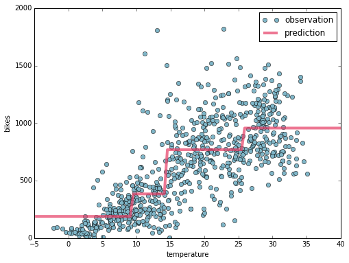
Decision Tree Regression
Here you can note that the prediction increases when the temperature increases. You can also note that the prediction is a stepwise function of the temperature. This is strictly related to how Decision Trees work. A decision tree splits the input features (only temperature in this case) in several regions and assigns a prediction value to each region. The selection of the regions and the predicted value within a region are chosen in order to produce the prediction which best fits the data. Where for best fit we mean that it minimises the distance of the observations from the prediction.
You can inspect the set of rules created during the training process by exporting the tree:
from sklearn.tree import export_graphviz

export_graphviz(regressor, out_file='tree.dot', feature_names=['temperature'])
Here we exported the tree in dot format. Visualising it with Graphviz (http://www.graphviz.org/) we have the following result:
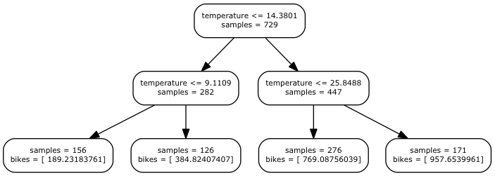
Decision Tree
The rules are organised in a binary tree: each time you ask to estimate the number of bikes hired the temperature is checked with the rules starting from the root of tree till the bottom following the path dictated form the outcome of the rules. For example, if the input temperature is 16.5, the first checked (temperature <= 14.3) will give a negative outcome leading us to its right child node in the next level of the tree (temperature <= 25.8), this time you will have a positive response and you will end in its left child. This node is a leaf, which means that it doesn't contain a rule but the value that you want to predict. In this case, it predicts 769 bikes.
Usually decision trees can be much deeper, and the deeper they are, the more complexity they are able to explain. In this case, a two level tree was configured using the parameter max_depth during the instantiation of the model.
Here's the notebook with the code and the data.
ABOUT THE AUTHOR

Giuseppe Vettigli
Giuseppe is a Data Scientist who has worked in both academia and the research industry for many years. His work focuses on the development of machine learning models and applications to make inferences from both structured and unstructured data. He also writes a blog about scientific computing and data visualization in Python: http://glowingpython.blogspot.com.